Querying Building-Specific Data
For column definitions, see Columns for Data Extracted from Buildings.
Querying Equipment
Using the API, we can retrieve the data from all the buildings that belong to our organization:
>>> # Get a list of all the buildings under your Organization
>>> pd.json_normalize(client.get_all_buildings())
    id  org_id             name  ... point_count info.note info
0   66       6   T`Challa House  ...          81            NaN
1  427       6  Office Building  ...        4219       NaN  NaN
2  428       6       Laboratory  ...        2206       NaN  NaN
3  429       6         Hogwarts  ...        4394       NaN  NaN
# Get a list of all the buildings under your Organization
get_buildings() %>% select_if(~ !any(is.na(.))) # select call drops columns with all NAs
#   id org_id            name         timezone status equip_count point_count
#1  66      2  T`Challa House America/New_York   LIVE          18         171
#2 427      6 Office Building America/New_York   LIVE         137        2422
#3 428      6      Laboratory America/New_York   LIVE         124        1658
#4 429      2     Residential America/New_York   LIVE         311        4394
The first column of this dataframe (id) contains the building identifier number.
In order to retrieve the equipment for a particular building (e.g. Laboratory, id: 428), we use get_building_equipment():
>>> # Get a list of all equipment in a building
>>> all_equipment = pd.DataFrame(client.get_building_equipment(428))
>>> all_equipment[['id', 'building_id', 'equip_id',  'points', 'tags']]
        id  building_id        equip_id                                             points                  tags
0    43342          428    fumeHood-409  [{'building_id': 428, 'description': 'Lab 409A...           [fan, hvac]
1    43076          428  meter-CHW Flow  [{'building_id': 428, 'description': 'GPM FLOW...        [water, meter]
2    27314          428  coolingTower-2  [{'building_id': 428, 'description': None, 'de...  [coolingTower, hvac]
3    33888          428           ahu-1  [{'building_id': 428, 'description': 'Exhaust ...           [ahu, hvac]
4    33889          428           ahu-2  [{'building_id': 428, 'description': 'Chilled ...           [ahu, hvac]
## TODO: make wrapper in R
Querying Specific Points
In order to query specific points, first we need to instantiate the PointSelector:
>>> from onboard.client.models import PointSelector
>>> query = PointSelector()
query <- PointSelector()
There are multiple ways to select points using the PointSelector. The user can select all the points that are associated with one or more lists containing any of the following:
'orgs', 'buildings', 'point_ids', 'point_names', 'point_hashes',
'point_topics', 'updated_since', 'point_types', 'equipment', 'equipment_types'
For example, here we make a query that returns all the points of the type ‘Real Power’ OR of the type ‘zone_air_temperature_sensor’ that belong to the ‘Laboratory’ building:
>>> query = PointSelector()
>>> query.point_types = ['zone_air_temperature_sensor']
>>> query.buildings = ['Laboratory']
>>> selection = client.select_points(query)
query <- PointSelector()
query$point_types <- c('zone_air_temperature_sensor')
query$buildings <- c('Laboratory')
selection <- select_points(query)
We can add to our query to e.g. further require that returned points must be associated with the ‘HVAC/FCU’ equipment type:
>>> query = PointSelector()
>>> query.point_types = ['zone_air_temperature_sensor']
>>> query.equipment_types = ['HVAC/FCU']
>>> query.buildings = ['Laboratory']
>>> selection = select_points(query)
>>> selection
{'orgs': [6],
'buildings': [428],
'equipment': [27356, 27357],
'equipment_types': [102],
'point_types': [2044],
'points': [289701, 289575]}
query <- PointSelector()
query$point_types <- c('zone_air_temperature_sensor')
query$equipment_types <- c('HVAC/FCU')
query$buildings <- c('Laboratory')
selection <- select_points(query)
selection
$orgs
[1] 6

$buildings
[1] 428

$equipment
[1] 27356 27357

$equipment_types
[1] 9

$point_types
[1] 77

$points
[1] 289701 289575
In this example, the points with ID=289701, and 289575 are the only ones that satisfy the requirements of our query.
We can get more information about these points by calling the function get_points_by_ids() on the points field in the selection entity:
>>> # Get metadata for the sensors you would like to query
>>> sensor_metadata = client.get_points_by_ids(selection['points'])
>>> sensor_metadata_df = pd.DataFrame(sensor_metadata)
>>> sensor_metadata_df[['id', 'building_id', 'first_updated', 'last_updated', 'type', 'value', 'units']]
       id  building_id  first_updated  last_updated                         type value              units
0  289575          428   1.626901e+12  1.724094e+12  zone_air_temperature_sensor  78.0  degreesFahrenheit
1  289701          428   1.626901e+12  1.724094e+12  zone_air_temperature_sensor  76.0  degreesFahrenheit
# Get metadata for the sensors you would like to query
sensor_metadata_df <- get_points_by_ids(selection$points) %>%
    select(id, building_id, first_updated, last_updated, type, value, units)
#      id building_id first_updated last_updated             type value             units
#1 289575         428  1.626901e+12 1.669934e+12 zone_air_temperature_sensor  68.0 degreesFahrenheit
#2 289701         428  1.626901e+12 1.669934e+12 zone_air_temperature_sensor  64.0 degreesFahrenheit
sensor_metadata_df now contains a dataframe with rows for each point. Based on the information about these points, we can observe that none of the points of our list belongs to the point type ‘Real Power’, but only to the point type ‘zone_air_temperature_sensor’
Exporting Data to .csv
Data extracted using the API can be exported to a .csv or excel file like so:
>>> # Save metadata to .csv file
>>> sensor_metadata_df.to_csv('./metadata_query.csv')
# Save metadata to .csv file
write.csv(sensor_metadata_df, file = "./metadata_query.csv")
Querying Time-Series Data
To query time-series data first we need to import relevant helper modules/packages.
>>> from datetime import datetime, timezone, timedelta
>>> import pytz
>>> from onboard.client.models import TimeseriesQuery, PointData
>>> from onboard.client.dataframes import points_df_from_streaming_timeseries
# install.packages('lubridate') # install if you haven't already
library(lubridate)
We select the range of dates we want to query, making sure to specify timezones:
>>> start = pd.Timestamp("2022-03-29 00:00:00", tz="utc")
>>> end = pd.Timestamp("2022-07-29 00:00:00", tz="utc")
start <- as_datetime("2022-03-29 00:00:00", tz = "UTC")
end <- as_datetime("2022-07-29 00:00:00", tz = "UTC")
Now we are ready to query the time-series data for the points we previously selected in the specified time-period:
>>> # Get time series data for the sensors you would like to query
>>> timeseries_query = TimeseriesQuery(point_ids = selection['points'], start = start, end = end)
>>> sensor_data = points_df_from_streaming_timeseries(client.stream_point_timeseries(timeseries_query))
>>> sensor_data
                         timestamp  289575 289701
0      2022-01-04T19:34:11.741000Z  NaN   60.0
1      2022-01-04T19:34:19.143000Z  62.0  NaN
2      2022-01-04T19:35:12.133000Z  NaN   60.0
sensor_data <- get_timeseries(start_time = start, end_time = end, point_ids = selection$points) #Queries timeseries data for the selection list we
sensor_data
#   timestamp           `289575` `289701`
#   <dttm>                 <int>    <int>
#1  2022-03-29 00:00:24       62       NA
#2  2022-03-29 00:01:25       62       NA
#3  2022-03-29 00:02:26       62       NA
Your time-series data will default to the units specified in https://portal.onboarddata.io/account?tab=unitPrefs, which can be set for your account or for all users in your organization. You can also specify your preferred units for each measurement type directly:
>>> # Get time-series data with chosen units
>>> timeseries_query = TimeseriesQuery(point_ids = selection['points'], start = start, end = end, units = {'pressure':'inH2O'})
# Get time-series data with chosen units
units <- data.frame("temperature" = "k")
timeseries <- get_timeseries(start_time, end_time, point_ids, units)
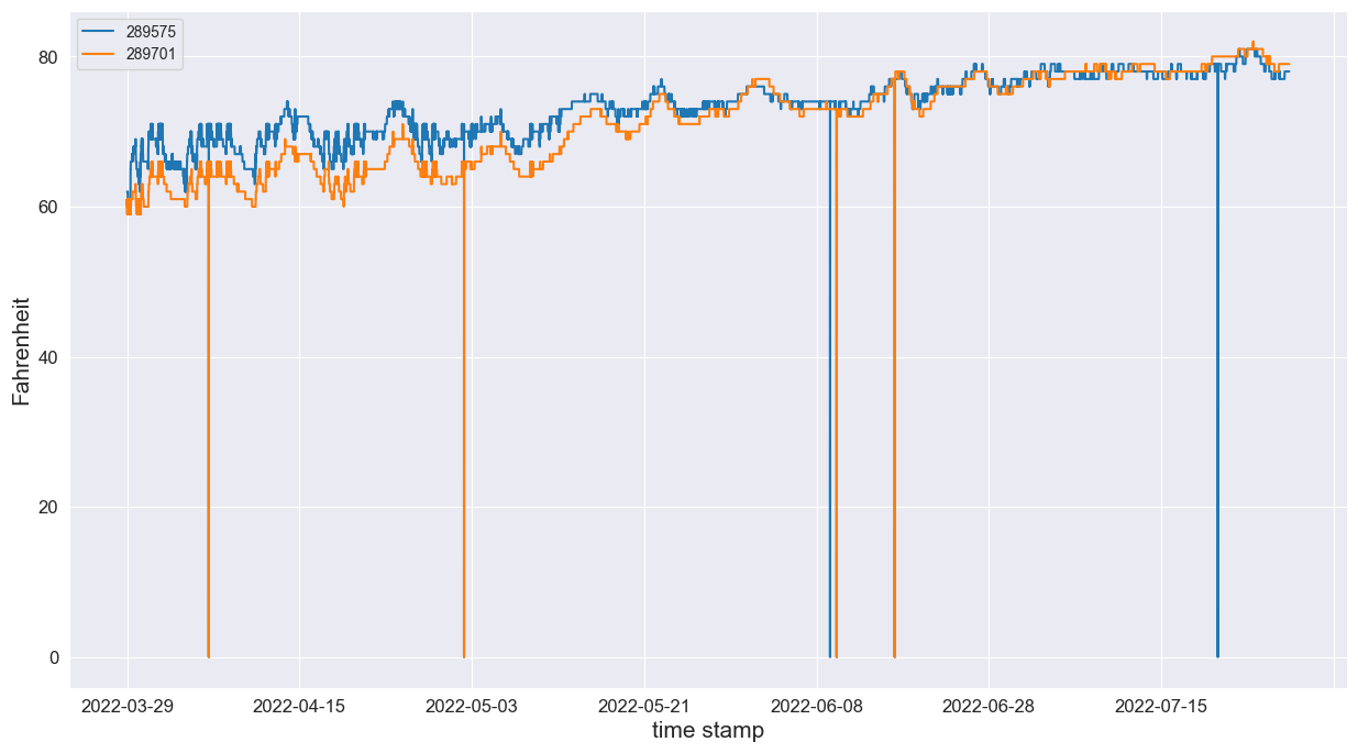
This returns a dataframe containing columns for the timestamp and for each requested point. And now we can plot these data:
>>> # set the timestamp as the index and forward fill the data for plotting
>>> sensor_data_clean = sensor_data.set_index('timestamp').astype(float).ffill()
>>>
>>> # Edit the indexes just for visualization purposes
>>> indexes = [i.split('T')[0] for i in list(sensor_data_clean.index)]
>>> sensor_data_clean.index = indexes
>>>
>>> fig = sensor_data_clean.plot(figsize=(15,8), fontsize = 12)
>>>
>>> # Adding some formatting
>>> fig.set_ylabel('Farenheit',fontdict={'fontsize':15})
>>> fig.set_xlabel('time stamp',fontdict={'fontsize':15})
>>> plt.show()
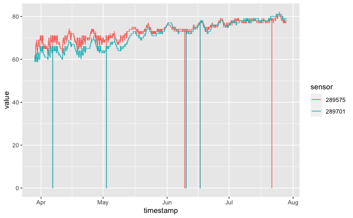
library(tidyverse)
# now, wrangle to tidy format:
sensor_data_clean <- sensor_data %>%
      mutate(timestamp = floor_date(timestamp, unit = "seconds")) %>%
      pivot_longer(-timestamp, names_to = "sensor", values_to = "value") %>%
      drop_na(value) %>%
      arrange(timestamp)
# and plot:
sensor_data_clean %>%
      ggplot(aes(x = timestamp, y = value, color = sensor)) +
      geom_line()